梯度法_共轭梯度法_线搜索

文章来自微信公众号“科文路”，欢迎关注、互动。转发须注明出处。

介绍了三种常用最优化方法，并使用Python进行了实验对比。

1 问题提出

https://en.wikipedia.org/wiki/Gradient_descent#Python

$$\min_{x} f(x)=x^4-3x^3+2$$

2 梯度法

2.1 梯度下降法 simple gradient method

https://en.wikipedia.org/wiki/Gradient_descent#Python

梯度下降法的思想很简单，每次下降方向选择梯度反方向，这样能保证每次值都在减小。
$$\begin{cases} x^{k+1}=x^k+\alpha d^k\d^k=-g^k\end{cases}$$

但问题是“锯齿”现象，所以效果很差，实际情况中一般不用。

x_k = 6 # The algorithm starts at x=6
alpha = 0.01 # step size multiplier
precision = 0.00001 # end mark
previous_step_size = 1 
max_iters = 10000 # maximum number of iterations
iters = 0 #iteration counter

df = lambda x: 4 * x**3 - 9 * x**2

while previous_step_size > precision and iters < max_iters:
    prev_x_k = x_k
    g_k = df(prev_x_k)
    d_k = -g_k
    x_k += alpha * d_k
    previous_step_size = abs(x_k - prev_x_k)
    iters+=1

print("The local minimum occurs at", x_k)
print("The number of iterations is", iters)

The local minimum occurs at 2.2499646074278457
The number of iterations is 70

2.2 共轭梯度法 conjugate gradient method

https://en.wikipedia.org/wiki/Conjugate_gradient_method

该方法基于梯度下降法。

由于梯度下降法每次下降的方向为负梯度方向，这并不能保证其是最优的方向。通过共轭方向的计算，保证第二步开始的下降方向在一个圆锥内，这能极大的提高下降的效率。

即
$$\begin{cases} x^{k+1}=x^k+\alpha d^k\d^k=-g^k+\beta d^k \ \beta = \frac{g_k^Tg_k}{g_{k-1}^Tg_{k-1}}\end{cases}$$

x_k = 6 # The algorithm starts at x=6
alpha = 0.01 # step size multiplier
precision = 0.00001 # end mark
previous_step_size = 1 
max_iters = 10000 # maximum number of iterations
iters = 0 #iteration counter
beta = 0

df = lambda x: 4 * x**3 - 9 * x**2

g_k = df(x_k)

while previous_step_size > precision and iters < max_iters:
    prev_x_k = x_k
    prev_g_k = g_k
    if 0 == iters:
        d_k = -g_k
    else:
        g_k = df(x_k)  
        beta = g_k*g_k/(prev_g_k*prev_g_k)
        d_k = -g_k + beta*d_k
    x_k += alpha * d_k
    previous_step_size = abs(x_k - prev_x_k)
    iters+=1

print("The local minimum occurs at", x_k)
print("The number of iterations is", iters)

The local minimum occurs at 2.2500110335395793
The number of iterations is 22

2.3 线搜索 line search

代码与例子来源于https://blog.csdn.net/u014791046/article/details/50831017

线搜加入了对步长的计算。

名为Backtracking Line Search(BLS)的梯度下降法以Armijo-Goldstein条件为方法，在以2.2为基础的搜索方向上选取不越过最优点的最大步长：

1. 定义$0<\beta<1$，及$0<\alpha\leq\frac{1}{2}$
2. 从$t=1$开始迭代$t=\beta t$，计算$$f(x_k-t\nabla f(x_k)) > f(x_k)-\alpha_k t|\nabla f(x_k)|_2^2$$

其中Armijo条件为
$$f(x_k+\alpha_kd_k) \leq f(x_k)+\alpha_k\beta\nabla f(x_k)^Td_k, where \beta \in (0,1)$$

# -*- coding: utf-8 -*-

# min 𝑓(𝑥)=(x-3)**2

import matplotlib.pyplot as plt

def f(x):
    '''The function we want to minimize'''
    
    return (x-3)**2
    
def f_grad(x):
    '''gradient of function f'''
    
    return (x-3)*2
 
    
x = 6
y = f(x)
MAX_ITER = 300
curve = [y]
i = 0
step = 0.1
previous_step_size = 1.0
precision = 1e-4

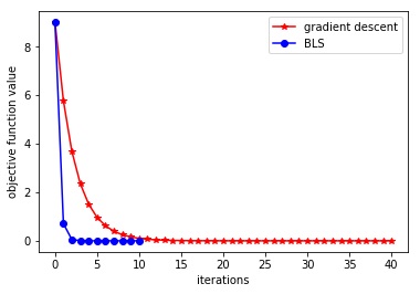
#下面展示的是我之前用的方法，看上去貌似还挺合理的，但是很慢
while previous_step_size > precision  and i < MAX_ITER:
    prev_x = x
    gradient = f_grad(x)
    x = x - gradient * step
    new_y = f(x)
    if new_y > y: #如果出现divergence的迹象，就减小step size
        step *= 0.8
    curve.append(new_y)
    previous_step_size = abs(x - prev_x)
    i += 1
     
print("The local minimum occurs at", x)
print("The number of iterations is", i)

plt.figure()
plt.show() 
plt.plot(curve, 'r*-')

plt.xlabel('iterations')
plt.ylabel('objective function value')
 
#下面展示的是backtracking line search，速度很快
x = 6
y = f(x)
alpha = 0.25
beta = 0.8
curve2 = [y]
i = 0
previous_step_size = 1.0
precision = 1e-4
 
while previous_step_size > precision  and i < MAX_ITER:
    prev_x = x
    gradient = f_grad(x)
    step = 1.0
    while f(x - step * gradient) > f(x) - alpha * step * gradient**2:
        step *= beta
    x = x - step * gradient
    new_y = f(x)
    curve2.append(new_y)
    previous_step_size = abs(x - prev_x)
    i += 1
    
print("The local minimum occurs at", x)
print("The number of iterations is", i)

plt.plot(curve2, 'bo-')
plt.legend(['gradient descent', 'BLS'])
plt.show()

运行结果如图

The local minimum occurs at 3.0003987683987354
The number of iterations is 40
<Figure size 432x288 with 0 Axes>
The local minimum occurs at 3.000008885903001
The number of iterations is 10

3 其他方法

其他方法还有如Riccati与Collocation，以后有时间再单独总结。

都看到这儿了，不如关注每日推送的“科文路”、互动起来~