独立成分分析ICA

文章来自微信公众号“科文路”，欢迎关注、互动。转发须注明出处。

在统计学中，独立成分分析或独立分量分析（Independent components analysis，缩写：ICA） 是一种利用统计原理进行计算的方法。它是一个线性变换。这个变换把数据或信号分离成统计独立的非高斯的信号源的线性组合。独立成分分析是盲信号分离（Blind source separation）的一种特例。

之前不太清楚这是什么，今天看到《机器学习工程师必知的十大算法》里这一条还没听过用过。而看了个大致介绍，感觉和我的毕设有点契合，所以集中学习一下。

0 参考资料

/wiki/Independent_component_analysis

独立成分分析法基本原理.pdf

ICA算法之算法实现

/ica-史上最直白的ICA教程.pdf

FastICA on 2D point clouds

百度百科-独立成分分析

1 简介

In signal processing, independent component analysis (ICA) is a computational method for separating a multivariate signal into additive subcomponents. This is done by assuming that the subcomponents are non-Gaussian signals and that they are statistically independent from each other. ICA is a special case of blind source separation.

中文不太好的维基：在统计学中，独立成分分析或独立分量分析（Independent components analysis，缩写：ICA） 是一种利用统计原理进行计算的方法。它是一个线性变换。这个变换把数据或信号分离成统计独立的非高斯的信号源的线性组合。独立成分分析是盲信号分离（Blind source separation）的一种特例。

2 定义

• 一句话，从多通道测量中得到的有若干独立信源线性组合成的观测信号中，将独立成分分解出来。
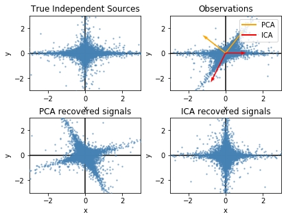
  • 因为主成分分析只对符合高斯分布的样本点比较有效，所以ICA可以看成是主成分分析与因子分析的延展。
• 
• 独立成分分析的最重要的假设就是信号源统计独立。这个假设在大多数盲信号分离的情况中符合实际情况。
  • 即使当该假设不满足时，仍然可以用独立成分分析来把观察信号统计独立化，从而进一步分析数据的特性。
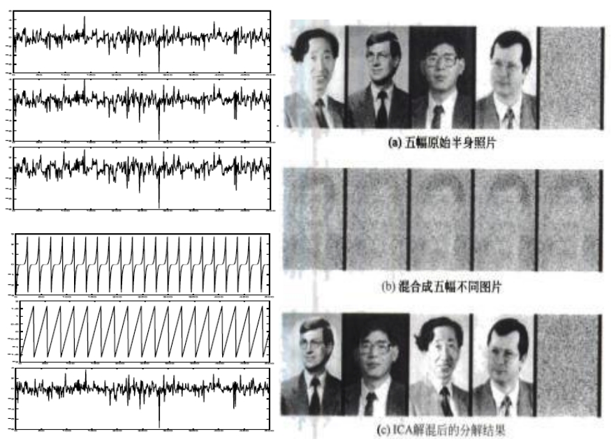
• 独立成分分析的经典问题是“鸡尾酒会问题”（cocktail party problem）。
  • 该问题描述的是给定混合信号，如何分离出鸡尾酒会中同时说话的每个人的独立信号。
  • An important note to consider is that if $N$ sources are present, at least $N$ observations (e.g. microphones if the observed signal is audio) are needed to recover the original signals. This constitutes the case where the matrix is square ($D=J$ , where $D$ is the number of observed signals and $J$ is the number of source signals hypothesized by the model). Other cases of underdetermined ($D<J$) and overdetermined ($D>J$) have been investigated.
    • 当有$N$个信号源时，通常假设观察信号也有$N$个（例如$N$个麦克风或者录音机）。该假设意味着混合矩阵是个方阵，即$J = D$，其中$D$是输入数据的维数，$J$是系统模型的维数。对于$J < D$和$J > D$的情况，学术界也分别有不同研究。
  • 独立成分分析并不能完全恢复信号源的具体数值，也不能解出信号源的正负符号、信号的级数或者信号的数值范围。

2.1 问题分类

Linear independent component analysis can be divided into noiseless and noisy cases, where noiseless ICA is a special case of noisy ICA. Nonlinear ICA should be considered as a separate case.

2.2 General definition

The data are represented by the observed random vector ${\boldsymbol {x}}=(x_{1},\ldots ,x_{m})^{T}$ and the hidden components as the random vector ${\boldsymbol {s}}=(s_{1},\ldots ,s_{n})^{T}.$ The task is to transform the observed data using a linear static transformation ${\boldsymbol {W}}$ as ${\boldsymbol {s}}={\boldsymbol {W}}{\boldsymbol {x}}$, into an observable vector of maximally independent components ${\boldsymbol {s}}$ measured by some function $F(s_{1},\ldots ,s_{n})$ of independence.

简单讲，就将观察到的向量通过线性变换，使其本身的隐含成分的独立成分被分离。

2.3 Generative model

2.3.1 Linear noiseless ICA

The components $x_{i}$ of the observed random vector ${\boldsymbol {x}}=(x_{1},\ldots ,x_{m})^{T}$ are generated as a sum of the independent components $s_{k}$, $k=1,\ldots ,n$:

$$
x_{i}=a_{i,1}s_{1}+\cdots +a_{i,k}s_{k}+\cdots +a_{i,n}s_{n}
$$
weighted by the mixing weights $a_{i,k}$.

The same generative model can be written in vector form as $\boldsymbol{x}=\sum_{k=1}^{n} s_{k} \boldsymbol{a}{k}$, where the observed random vector ${\boldsymbol {x}}$ is represented by the basis vectors $\boldsymbol{a}{k}=\left(\boldsymbol{a}{1, k}, \ldots, \boldsymbol{a}{m, k}\right)^{T}$.

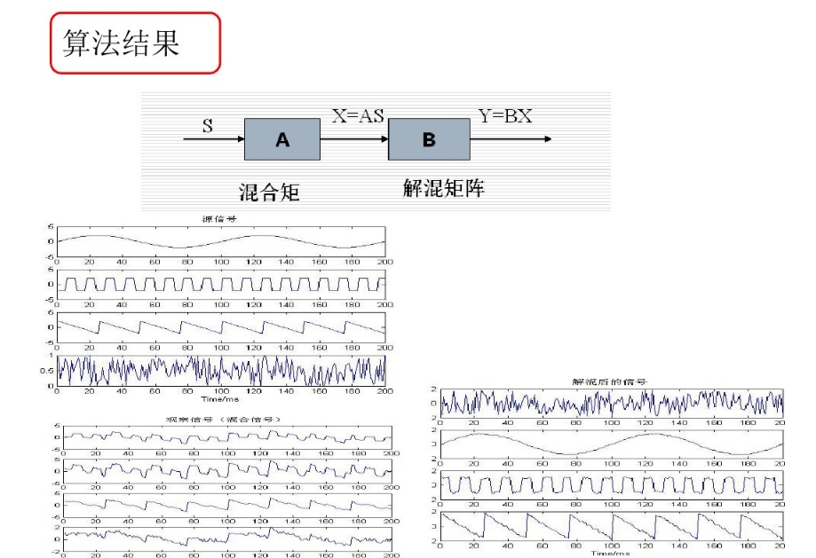
The basis vectors $\boldsymbol{a}{k}$ form the columns of the mixing matrix $\boldsymbol{A}=\left(\boldsymbol{a}{1}, \ldots, \boldsymbol{a}{n}\right)$ and the generative formula can be written as $\boldsymbol{x}=\boldsymbol{A} \boldsymbol{s}$, where $\boldsymbol{s}=\left(s{1}, \dots, s_{n}\right)^{T}$.

2.3.2 Linear noisy ICA

With the added assumption of zero-mean and uncorrelated Gaussian noise $n \sim N(0, \operatorname{diag}(\Sigma))$, the ICA model takes the form $\boldsymbol{x}=\boldsymbol{A} \boldsymbol{s}+\boldsymbol{n}$.

2.3.3 Nonlinear ICA

The mixing of the sources does not need to be linear. Using a nonlinear mixing function $f( \cdot| \theta)$ with parameters $\theta$ the nonlinear ICA model is $x=f(s | \theta)+n$.

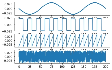
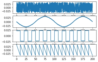
3 实战

操作上的感觉是这样的，

图/百度百科

独立成分分析存在各种不同先验假定下的求解算法。而且，经过ICA处理后，重建的数据幅度可能发生变化，自身也可能翻转。

fastica是sklearn.decomposition下的算法。

Implemented using FastICA: A. Hyvarinen and E. Oja, Independent Component Analysis: Algorithms and Applications, Neural Networks, 13(4-5), 2000, pp. 411-430

前提： 观测数据为数个独立、非高斯信号的线性组合。

此外，白化的意思是，使用白化矩阵消除各观测间的二阶相关性。这可以有效地降低问题的复杂度，而且算法简单，用传统的PCA就可完成。

对于sklearn，我看到了两个包，

• decomposition.FastICA([n_components, …]): FastICA: a fast algorithm for Independent Component Analysis.
• decomposition.fastica(X[, n_components, …]): Perform Fast Independent Component Analysis.

其步骤为

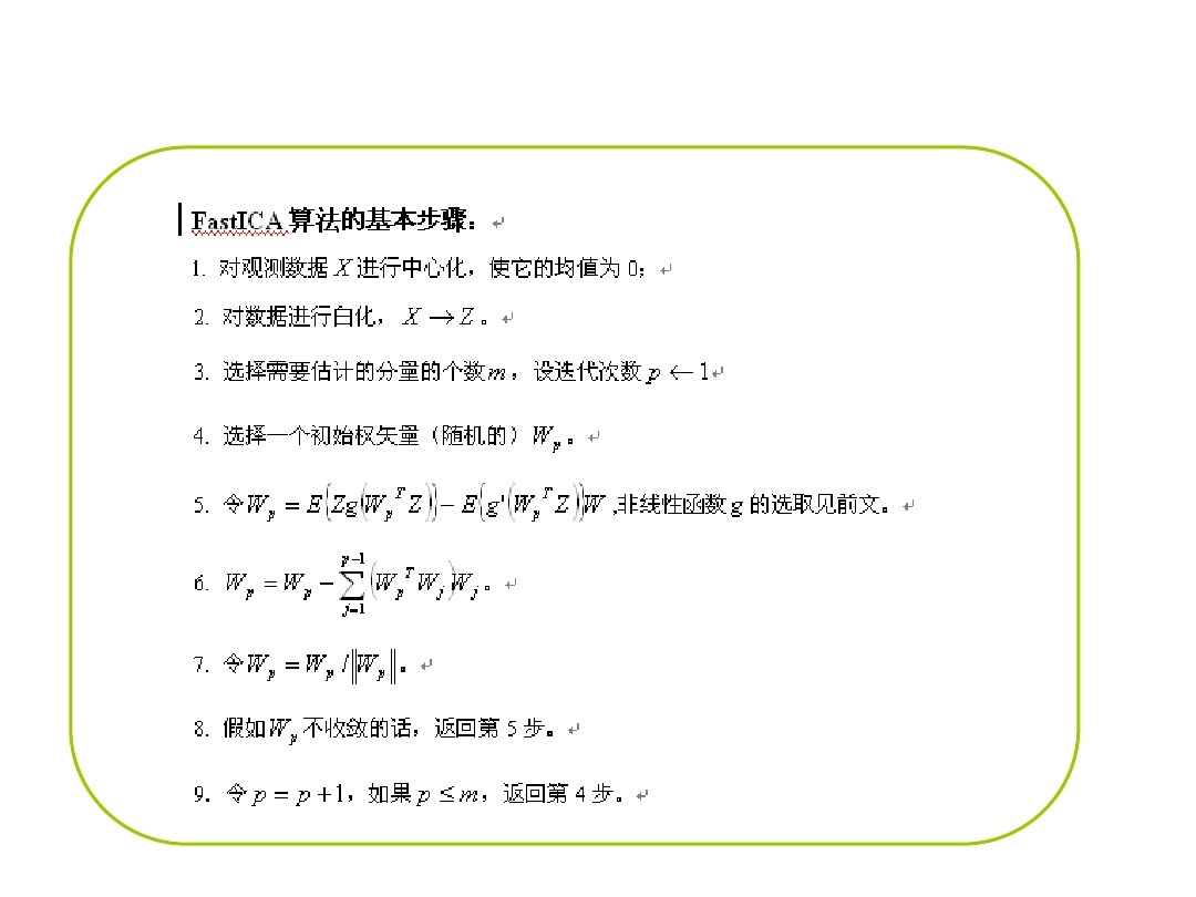
下面先看FastICA的示例，

3.1 FastICA on 2D point clouds (sklearn examples)

# -*- coding: utf-8 -*-

print(__doc__)

# Authors: Alexandre Gramfort, Gael Varoquaux
# License: BSD 3 clause

import numpy as np
import matplotlib.pyplot as plt

from sklearn.decomposition import PCA, FastICA

# #############################################################################
# Generate sample data
rng = np.random.RandomState(42)
S = rng.standard_t(1.5, size=(20000, 2))
S[:, 0] *= 2.

# Mix data
A = np.array([[1, 1], [0, 2]])  # Mixing matrix

X = np.dot(S, A.T)  # Generate observations

pca = PCA()
S_pca_ = pca.fit(X).transform(X)

ica = FastICA(random_state=rng)
S_ica_ = ica.fit(X).transform(X)  # Estimate the sources

S_ica_ /= S_ica_.std(axis=0)


# #############################################################################
# Plot results

def plot_samples(S, axis_list=None):
    plt.scatter(S[:, 0], S[:, 1], s=2, marker='o', zorder=10,
                color='steelblue', alpha=0.5)
    if axis_list is not None:
        colors = ['orange', 'red']
        for color, axis in zip(colors, axis_list):
            axis /= axis.std()
            x_axis, y_axis = axis
            # Trick to get legend to work
            plt.plot(0.1 * x_axis, 0.1 * y_axis, linewidth=2, color=color)
            plt.quiver(0, 0, x_axis, y_axis, zorder=11, width=0.01, scale=6,
                       color=color)

    plt.hlines(0, -3, 3)
    plt.vlines(0, -3, 3)
    plt.xlim(-3, 3)
    plt.ylim(-3, 3)
    plt.xlabel('x')
    plt.ylabel('y')

plt.figure()
plt.subplot(2, 2, 1)
plot_samples(S / S.std())
plt.title('True Independent Sources')

axis_list = [pca.components_.T, ica.mixing_]
plt.subplot(2, 2, 2)
plot_samples(X / np.std(X), axis_list=axis_list)
legend = plt.legend(['PCA', 'ICA'], loc='upper right')
legend.set_zorder(100)

plt.title('Observations')

plt.subplot(2, 2, 3)
plot_samples(S_pca_ / np.std(S_pca_, axis=0))
plt.title('PCA recovered signals')

plt.subplot(2, 2, 4)
plot_samples(S_ica_ / np.std(S_ica_))
plt.title('ICA recovered signals')

plt.subplots_adjust(0.09, 0.04, 0.94, 0.94, 0.26, 0.36)
plt.show()

3.2 网友的fastICA

# -*- encoding:utf-8 -*-

import sys
import math
import numpy as np
from matplotlib import pyplot as plt
from sklearn.decomposition import fastica
from copy import deepcopy


class ICA():
    def __init__(self, signalRange, timeRange):
        # 信号幅度
        self.signalRange = signalRange
        # 时间范围
        self.timeRange = timeRange
        # 固定每个单位时间10个点,产生x
        self.x = np.arange(0, self.timeRange, 0.1)
        # 所有的点数
        self.pointNumber = self.x.shape[0]

    # 生成正弦波
    def produceSin(self, period=100, drawable=False):
        y = self.signalRange * np.sin(self.x / period * 2 * np.pi)
        if drawable:
            plt.plot(self.x, y)
            plt.show()

        return y

    # 生成方波
    def produceRect(self, period=20, drawable=False):
        y = np.ones(self.pointNumber) * self.signalRange
        begin = 0
        end = self.pointNumber
        step = period * 10
        mid = step // 2
        while begin < end:
            y[begin:mid] = -1 * self.signalRange
            begin += step
            mid += step
        if drawable:
            plt.plot(self.x, y)
            plt.show()

        return y

    # 生成三角波
    def produceAngle(self, period=20, drawable=False):
        lastPoint = period * 10 - 1
        if lastPoint >= self.pointNumber:
            raise ValueError('You must keep at least one period!')
        delta = ((-1 - 1) * self.signalRange) / float(self.x[lastPoint] - self.x[0])
        y = (self.x[:lastPoint+1] - self.x[0]) * delta + self.signalRange
        y = np.tile(y, self.pointNumber // y.shape[0])[:self.pointNumber]

        if drawable:
            plt.plot(self.x, y)
            plt.show()
        return y

    # 生成uniform噪声
    def produceNoise(self, signalRange=None, drawable=False):
        if signalRange is None:
            signalRange = self.signalRange
        y = np.asarray([(np.random.random() - 0.5) * 2 * signalRange for _ in range(self.pointNumber)])

        if drawable:
            plt.plot(self.x, y)
            plt.show()

        return y

    # 混合信号
    def mixSignal(self,majorSignal, *noises, **kwargs):
        mixSig = deepcopy(majorSignal)
        noiseRange = 0.5
        if 'noiseRange' in kwargs and kwargs['noiseRange']:
            noiseRange = kwargs['noiseRange']
        for noise in noises:
            mixSig += noiseRange * np.random.random() * noise
        if 'drawable' in kwargs and kwargs['drawable']:
            plt.plot(self.x, mixSig)
            plt.show()

        return mixSig
        

    # 让每个信号的样本均值为0,且协方差(各个信号之间)为单位阵
    def whiten(self, X):
        # 加None可以认为是将向量进行转置,但是对于矩阵来说,是在中间插入了一维
        X = X - X.mean(-1)[:, None]
        A = np.dot(X, X.T)
        D, P = np.linalg.eig(A)
        D = np.diag(D)
        D_inv = np.linalg.inv(D)
        D_half = np.sqrt(D_inv)

        V = np.dot(D_half, P.T)

        return np.dot(V, X), V

    # 就是sklearn的源码里面的logcosh
    # 源码里有fun_args,用到一个alpha来调整幅度,这里省略没加
    # tanh(x)的导数为1-tanh(x)^2
    def _tanh(self, x):
        gx = np.tanh(x)
        g_x = gx ** 2
        g_x -= 1
        g_x *= -1
        return gx, g_x.mean(-1)

    def _exp(self, x):
        exp = np.exp(-(x ** 2) / 2)
        gx = x * exp
        g_x = (1 - x ** 2) * exp
        return gx, g_x.mean(axis=-1)


    def _cube(self, x):
        return x ** 3, (3 * x ** 2).mean(axis=-1)

    # W <- (W_1 * W_1')^(-1/2) * W_1
    def decorrelation(self, W):
        U, S = np.linalg.eigh(np.dot(W, W.T))
        U = np.diag(U)
        U_inv = np.linalg.inv(U)
        U_half = np.sqrt(U_inv)
        # rebuild_W = np.dot(np.dot(S * 1. / np.sqrt(U), S.T), W)
        rebuild_W = np.dot(np.dot(np.dot(S, U_half), S.T), W)
        return rebuild_W

    # fastICA
    def fastICA(self, X, fun='tanh'):
        n, m = X.shape
        p = float(m)
        if fun == 'tanh':
            g = self._tanh
        elif fun == 'exp':
            g = self._exp
        elif fun == 'cube':
            g = self._cube
        else:
            raise ValueError('The algorighm does not '
                             'support the support the user-defined function.'
                             'You must choose the function in (`tanh`, `exp`, `cube`)')
        # 不懂, 需要深挖才能知道, sklearn的源码里有这个,查的资料里说是black magic
        X *= np.sqrt(X.shape[1])

        # 随机化W,只要保证非奇异即可,源码里默认使用normal distribution来初始化,对应init_w参数
        W = np.ones((n,n), np.float32)
        for i in range(n):
            for j in range(i):
                W[i,j] = np.random.random()

        # 随机化W的另一种方法,但是这个不保证奇异
        # W = np.random.random((n, n))
        # W = self.decorrelation(W)

        # 迭代计算W
        maxIter = 300
        for ii in range(maxIter):
            gwtx, g_wtx = g(np.dot(W, X))
            W1 = self.decorrelation(np.dot(gwtx, X.T) / p - g_wtx[:, None] * W)
            lim = max(abs(abs(np.diag(np.dot(W1, W.T))) - 1))
            W = W1
            if lim < 0.00001:
                break
        return W

    # 画图
    def draw(self, y, figNum):
        if y.__class__ == list:
            m = len(y)
            n = 0
            if m > 0:
                n = len(y[0])
        elif y.__class__ == np.array([]).__class__:
            m, n = y.shape
        else:
            raise ValueError('The first arg you give must be type of list or np.array.')
        plt.figure(figNum)
        for i in range(m):
            plt.subplot(m, 1, i + 1)
            plt.plot(self.x, y[i])

    # 显示
    def show(self):
        plt.show()



if __name__ == '__main__':
    # 设置信号幅度为2,时间范围为[0, 200)
    ica = ICA(2, 200)
    # 周期为100的正弦波
    gsigSin = ica.produceSin(100, False)
    # 周期为20的方形波
    gsigRect = ica.produceRect(20, False)
    # 周期为20的三角波
    gsigAngle = ica.produceAngle(20, False)
    # 幅度为0.5的uniform噪声
    gsigNoise = ica.produceNoise(0.5, False)
    # 独立信号S
    totalSig = [gsigSin, gsigRect, gsigAngle, gsigNoise]
    # 混合信号X
    mixSig = []
    for i, majorSig in enumerate(totalSig):
        curSig = ica.mixSignal(majorSig, *(totalSig[:i] + totalSig[i+1:]), drawable=False)
        mixSig.append(curSig)
    mixSig = np.asarray(mixSig)


    # 以下是调用自己写的fastICA, 默认做了白化处理,不用白化效果貌似不太行
    xWhiten, V = ica.whiten(mixSig)
    # fun的选择和你假设的S的概率分布函数有关,一般假设为sigmoid函数, 则对应为tanh
    W = ica.fastICA(xWhiten, fun='tanh')
    recoverSig = np.dot(np.dot(W, V), mixSig)
# =============================================================================
#     ica.draw(totalSig, 1)
#     ica.draw(mixSig, 2)
# =============================================================================
    ica.draw(recoverSig, 3)
    ica.show()

    # 以下是调用sklearn包里面的fastICA
    # V对应白化处理的变换矩阵即Z = V * X, W对应S = W * Z
    V, W, S = fastica(mixSig.T)
    # 不做白化处理的话就不用乘K
# =============================================================================
#     assert ((np.dot(np.dot(W, V), mixSig) - S.T) < 0.00001).all()
# =============================================================================
# =============================================================================
#     ica.draw(totalSig, 1)
#     ica.draw(mixSig, 2)
# =============================================================================
    ica.draw(S.T, 3)
    ica.show()

4 应用

• optical Imaging of neurons
• neuronal spike sorting
• face recognition
• modelling receptive fields of primary visual neurons
• predicting stock market prices
• mobile phone communications
• color based detection of the ripeness of tomatoes
• removing artifacts, such as eye blinks, from EEG data.
• analysis of changes in gene expression over time in single cell RNA-sequencing experiments.
• studies of the resting state network of the brain.

都看到这儿了，不如关注每日推送的“科文路”、互动起来~